When engineering quantitative financial software to extract capital from public markets, statistical precision is paramount. Yet, when surveying various commercial platforms, it becomes clear that many fundamentally misunderstand central tendency and conflate secular drift with genuine calendar edge.
Most commercial tools present seasonality as the average or mean monthly return of an asset. This approach suffers from two fatal flaws:
- The Average/Mean vs. Median Trap: Averages are highly susceptible to outliers. A single exogenous shock—like the March 2020 pandemic crash—will drag the entire seasonal average down, generating false bearish signals for years to come. You are trading on echoes of 2020 which will never replay exactly the same.
- The Secular Trend Illusion: Commercial tools often confuse a macro compound annual growth rate (CAGR) with actual seasonality. If an asset is in a massive multi-year secular bull market, it will trend upward regardless of the calendar month. Highlighting that an asset is "up 70% of the time in September" is mathematically meaningless if the asset is up 70% of the time across all months due to secular drift.
To isolate true seasonal influences from random market noise and secular trends, ratioplotter.eu utilizes a strictly median-based daily aggregation, log-linear detrending, and out-of-sample validation. By the way: non-subscribers can plot 8 seasonality charts per month for free on our tool.
Dissecting the Seasonality Engine
The seasonality charts below are generated by an engine designed specifically for capital deployers, functioning not just as a historical visualizer, but as a rigorous backtester of calendar shape.
Seasonality Chart for ticker WOOD (iShares Global Timber & Forestry ETF). See URL for up-to-date version: https://ratioplotter.eu/seasonality.html?ta=T-WOOD-SplitAdjClose
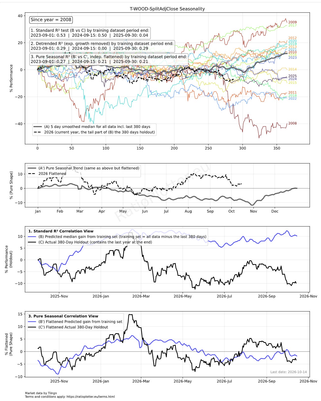
On the above analysis, the current year’s price gains is the dashed black line on the first and second panels from the top, and the continuous black line on the two panels at the bottom. The seasonal trend is the grey thick line on the top two panels, and the blue line on the bottom two panels. The four panels are necessary to remove noise and get to the pure seasonal trend. The first panel shows that the current year (dashed line) is below the secular and calendar trend (thick grey line), but when we get to the bottom truth of the last panel we see that the current year black line is actually above the calendar trend, the pure seasonal blue line.
The engine calculates normalized Year-To-Date (YTD) logic, plotting historical years as individual percentage deviations from their January 1st starting price (colored lines). Instead of averaging these years, it calculates the composite seasonality curve using the median, effectively discarding extreme outlier years (thick grey line on the top two panels and blue line on the bottom two panels).
Furthermore, the system is not limited to single tickers; it can process complex mathematical expressions and combinations of assets such as the seasonality of the ratio of two tickers.
The Out-of-Sample Holdout
To prevent "look-ahead bias"—the illusion of predictability caused by testing a model on the exact same data used to build it—the engine physically clamps the timeline. It hides the most recent 380 days from the mathematical engine, forcing the system to predict the hidden future using only older historical data. It runs this holdout test three consecutive times to ensure a single anomalous year does not artificially inflate the asset's predictive score.
From Noise to the Truth, The Three Tiers of Correlation (R²)
The engine scores predictive validity using three progressively stricter R² metrics:
- Standard R² (Raw Directional Accuracy): Measures the direct correlation between the predicted median gain and the actual holdout period. This score is easily inflated by secular baseline drift; if an asset compounds upward reliably, both lines drift up together, masking whether the calendar-specific peaks and troughs actually aligned.
- Detrended R²: Mathematically strips out the historical compound growth rate from both the prediction and the reality before scoring them.
- Pure Seasonal R² (Shape Correlation): The ultimate shape test. It neutralizes macroeconomic noise by using Ordinary Least Squares (OLS) and log-linear regression to independently level both the prediction and the actual holdout to a zero-slope horizontal axis. This extracts the “pure seasonal shape,” completely independent of the asset’s broader bull or bear environment.
Real-World Applications
iShares Global Timber & Forestry ETF (WOOD)
The ticker WOOD exhibited strong seasonality across recent years, likely driven by harvest periodicity and the rush from resellers to purchase inventory ahead of winter snows and spring builder demand.
The bottom panel of this chart demonstrates the “Pure Shape” isolation. By removing the mean exponential growth, we can observe the flattened seasonal shape. If standard commercial software analyzed this ticker, the secular growth would entirely obscure these specific harvest-cycle entry and exit points.
Global Equities: iShares MSCI World (URTH)
Equities often face a confluence of macroeconomic headwinds, from shifting CAPE ratios to anticipated rate hikes. In the absence of new fundamental information, we rely on seasonal models to gauge the statistical probabilities of price action.
Based on the last 14 years of URTH price history, the market typically experiences a minor structural spike just before mid-September (the thick grey line in the top panel). This is called by the investor community the September effect. However, the active year (the dotted black line) ignored this anticipated rally, trending flat-to-down since August.
When we isolate the Pure Seasonal R² for this asset, we see a value of 0.33 (see full article below):
Link for article: /articles/20260915_seasonality_T-URTH.html
This mathematically proves that on seasonal years around 25% to 27% of the price variance above the dominating exponential growth trend in the 380-day holdout window was driven purely by calendar effects.
If you are basing capital deployment on charts that calculate monthly averages and ignore the difference between secular momentum and true calendar variance, you are trading on noise. By demanding median aggregations, daily tracking, and out-of-sample holdout validation, you ensure your seasonal models possess genuine predictive edge.
Final disclaimer: for informational purposes only. Not investment advice or a recommendation. Investing involves risk. Reading this publication does not create an advisory relationship.