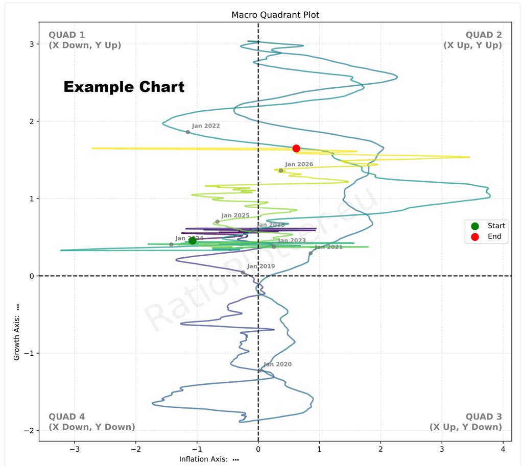
Macro Quadrant Trajectory Plot
Visualize chronological changes mapping rate of change for X-Axis (Typically Inflation) vs Y-Axis (Typically Growth) through the four major economic regimes.
Interpretation and strategic portfolio positioning: We do not provide investment advice, only educational and analytics tools and material. To understand the different charts, I advise you to read, ask experets, and ask AI about how a portfolio could be positioned for the different economic regimes from the quadrants above.
Maybe this prompt is useful as start: Regarding economic regime macro quadrant charts ploting the <substitute your x axis and y axis here: rate of change of inflation and growth>. Can you explain which assets are interesting to buy or sell on each quadrant and why? By quadrants I mean Q1, Q2, Q3, Q4 as defined above, with Q1 being y up, x down; and Q2 being y up and x up; and Q3 y down and x up; and Q4 being y down and x down? Do the quadrants have names for the specific x and y given?
We also add that there are two typical ways to position yourself regarding these quadrant transitions. One way is to position yourself for a momentum play, this is usually the case when for instance when one variable is already rising such as inflation and you trade to take advantage that it will continue to rise after all the acceleration is positive. Such a play could involve for instance buying commodities that readjust their prices for inflation (depends also on the economic growth trend). Another way is to position yourself is not on a momentum play, but on a mean reversal play, this is usually the case when the trajectory is likely to reverse to the mean and oscillate, cross to the other side of the x or y axis. For instance, inflation, and commodities may have started changing from negative acceleration to positive and you could position for a reversal by accumulating commodities at ever lower prices. Here the analysis of an overlay plot and how deep the lows in commodity prices could be useful, it is for instance interesting to buy cotton, sugar, oil below the production price for some countries.
Suggested Quadrant Plot Trajectories (Free Tier)
Trading Notes & Guide
Help & Notes
Z scaling, standardization: Feel free to remove the Z_SCALE call and see inflation acceleration not in the normal curve scale, but in the physics scale for acceleration points.
Common Start Date: The chart automatically finds the earliest date where all requested tickers have valid data (the intersection). Any data prior to this "Common Start" is trimmed to ensure a fair comparison.
Limit: The Free Tier is restricted to specific pre-defined baskets arguments for this chart, advanced users (subscribers) can enter any argument they wish, we use T-COM as a proxy for worldwide inflation.
Ticker Data Usage, Data Sourcing and Ticker Functions
Ticker Data Sources
Default Ticker Column Projections & Adjustments
ADD() Element-wise adding
ADD(T-AAPL, T-MSFT) or ADD(T-GLD, 10.5).
CLOSE_GAPS() Interpolating and extrapolating sparse data
CLOSE_GAPS(ES-teicp000-coicop18, 'LINEAR', 'FORWARD_FILL', 60).
Our tickers are all by default forward filled in their gaps (non-data non-trading days), except for IMF- tickers
which are linearly interpolated and for ES- tickers which do not have their gaps closed at all. To change the
default gap closing applied, simply wrap the ticker in CLOSE_GAPS to apply a new strategy to close the data gaps.
For instance FED-WPU53 is by default forward-filled, to change it to linear interpolated with zero days extrapolated,
write it as:
CLOSE_GAPS(FED-WPU53, 'LINEAR', 'LINEAR', 0)
CURVE_FROM_VECTOR() Custom data vectors
CURVE_FROM_VECTOR([198.27, 211.92, 245.12, 281.72, 318.27], '2026-06-30', 'last', '1y', 'linear', 'forward_fill').
Arguments represent the array of values, anchor date, anchor position ('first' or 'last'), frequency ('1y', '1q', '1m'), interpolation ('linear', 'forward_fill'), and extrapolation ('none', 'forward_fill', 'linear').
LAG() Time-shifted underlying vector
LAG(T-AAPL, 10). It is highly useful for autocorrelation studies.
LINEAR_COMBINATION() Weighted sum of multiple vectors
LINEAR_COMBINATION([1.5, -0.5], [T-AAPL, T-MSFT]).
LOG() Logarithmic transformation
LOG(T-GOOGL, 2) or LOG(T-MSFT, 10). If you want you can use EPSILON constant which is not a natural logarithm constant, but just a logarithm on a tiny base: LOG(T-SPY, EPSILON). We encourage using LOG on the base two as it is the fastest to compute for you and will allow caching of the computation for others to benefit.
The LOG on base 2 will also mean you are measuring how long it takes for the time series to double, a difference in 1 point is a doubling.
LOOK_FORWARD() Shifting data forward in time
LOOK_FORWARD(T-AAPL, 30).
The second argument 30 is the number of days to look forward. All our data for time series is measured in days.
MATH- Custom Mathematical Tickers
MINUS() Element-wise subtraction
MINUS(T-AAPL, T-MSFT).
MOVING_AVERAGE() Trailing Simple Moving Average
MOVING_AVERAGE(T-SPY, 200) calculates the 200-day trailing moving average.
MULT() Element-wise multiplication
MULT(T-COM, T-USDCHF)
performs a currency conversion of the T-COM broad commodity investment basket to Swiss Francs (most of our tickers are in USD and that
ticker price currency can be seen on the ticker selector page). T-COM is the: DIREXION AUSPICE BROAD COMMODITY STRATEGY ETF.
RAT() Calculating Ratio Between Two Tickers
RAT(T-AAPL, T-MSFT). Example of comparing Google's outperformance to an idealized
CAGR curve: RAT(T-GOOGL,T-MSFT)/MATH-CAGR_PCT-2 (requires login with Google).
REGRESSION() and RESIDUALS() Functions
(1) The REGRESSION or RESIDUAL functions are reserved for paying users, apart from the free tier REGRESSION examples present on the log plot page.
(2) When the REGRESSION() function is the outermost function of the expression and is used on the log plotter, it will cause a nice regression plot canvas to display the fitting line and useful regression statistics such as ADF probability and R².
If used on the regular ratio plotter page, it will plot the residuals vector. Example: REGRESSION(LOG(T-URTH,2)) (this example requires subscription as it uses the LOG function).
The REGRESSION function is very good at modelling time series that grow following a linear trend. Most financial assets grow following an exponential trend, which means that if we apply the LOG function to this asset ticker we obtain a linear trend which can be modelled by the REGRESSION function. Try it, try plotting just LOG(T-GOOGL) to see this straight line tendency.
RET() Rolling Percentage Return
RET(T-SPY, 30)
measures the rolling 30-day percentage performance. The return for a day is always measured looking back
at the last x days (30 in the example), otherwise we would introduce look-ahead bias into our models of returns.
To calculate forward returns you can combine the two functions RET(LOOK_FORWARD(T-GOOGL,30),30). Easy right?
ROLLING_SLOPE() Calculating slope, velocity, or derivating
ROLLING_SLOPE(IMF-NGDPD-CHN, 400, 1). The second argument (400) is the lookback
window in days to calculate the smoothed slope. The third argument (1) determines the scalar output
granularity (e.g., 1 for daily velocity, 365 to annualize the velocity).
Example: China GDP Velocity.
SIMUL_TICKER_DIV_REINVEST() Plotting Dividends Reinvested at Your Portfolio Return Rate
SIMUL_TICKER_DIV_REINVEST(T-MSFT,0.25,1,'2022-08-01').
This is a function available only for users with the advanced subscription. The first argument is the
Ticker simulated, the second is your portfolio CAGR rate (in this case 0.25 = 25% yoy, applied dynamically daily).
The third argument is the initial investment in the currency of the stock ticker. The last argument is the
start date. See our article on dividend reinvestment simulation.
VOLATILITY() Annualized Rolling Volatility
VOLATILITY(T-SPY, 50) measures the annualized volatility of
the S&P 500 utilizing a 50-day rolling lookback window. The Scatter plot tool
has some examples of the VOLATILITY function.
Z_SCALE() Z scaling, bringing data to the normal curve Z score scale, normalizing
Z_SCALE(T-MSFT),
Z_SCALE(RAT(T-GLD,T-SLV)), Z_SCALE(ROLLING_SLOPE(T-COM,90,1)). This brings
absolute price vectors or ratios to a standardized Normal Curve (Mean 0, StdDev 1) for macro-economic
cycle alignment. This function is available only for users with the advanced subscription.
The Buffett Indicators Tool allows plotting the Z-Scale spread
of the country ETF price to its GDP figures.