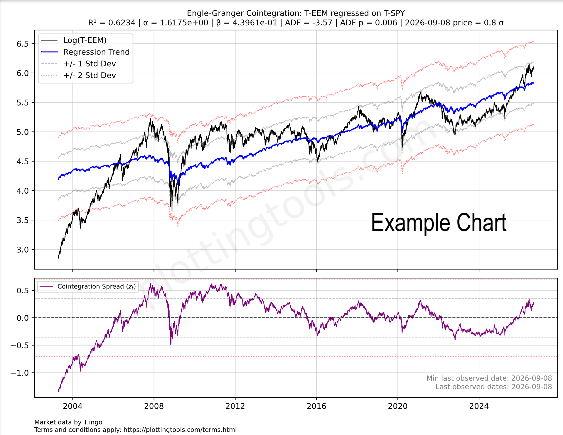
Engle-Granger Cointegration Builder
In simple terms, Engle-Granger models allow predicting an asset price based on the price of another asset. If you'd like a more elaborate description: Engle-Granger allows constructing the optimal hedge ratio regression and plotting the resulting stationary portfolio. To learn more about how to use Engle-Granger we recommend our article: Is AI impacting India's Economy.
Engle-Granger Cointegrating Regression (Formula on Formula)
Unlike the constrained ratio spread (which forces a 1-to-1 relationship), this regression estimates the optimal empirical hedge ratio ($\beta$) between the two assets to create a stationary portfolio. In statistical arbitrage, $\beta$ dictates exactly how much of tickerb you should short for every unit of tickera you buy to remain market-neutral.
The LaTeX Equation for the fans: $$\log_2(P_{a,t}) = \alpha + \beta \log_2(P_{b,t}) + \epsilon_t$$ $\beta$ is the unconstrained hedge ratio (the cointegrating coefficient).
$\epsilon_t$ represents the spread (the residuals). If the two tickers are genuinely cointegrated, this $\epsilon_t$ series will be mean-reverting.
Engle-Granger Plots (Free Demos and Paid)
Below we have some plot suggestions of ticker pairs for Engle-Granger cointegration. For the rank of best Engle-Granger regressions see:: Insights on the Best Engle Granger Regressions. The ADF and ADF p noted on the suggestions are from 2026-09-10, click on the plot for a fresh ADF-p estimate.
Trading Notes & Guide
General Notes
Currency Consistency: Ensure tickers are in the same currency to avoid exchange rate noise affecting the ratio.
See the currency on the Ticker Selector Page.
ETF Consistency: When plotting the ratio between two ETF's, always check that both are either distributing or accumulating. If this is not the case dividends can effect the results significantly!
R2 and ADF p: Ensure the R2 and ADF p point to a good quality model which can be used for trading (see table below).
Recommendation: Always check the seasonality plot of the ticker you intend to swing trade; ensure the historical seasonality isn't moving against your position.
Online Engle-Granger Cointegration for Pairs Trading
The Engle-Granger Two-Step Method is the foundational econometric model for pairs trading and statistical arbitrage. While simple ratio spreads (like our Constrained Ratio Spread model) force a 1:1 relationship between two assets, this online Engle-Granger cointegration tool uses Ordinary Least Squares (OLS) regression to calculate the optimal hedge ratio ($\beta$) dynamically. This allows you to construct a perfectly market-neutral, stationary portfolio even if the assets have drastically different volatilities or dollar values.
Here is how our engine executes the two steps:
- Step 1 (The Cointegrating Regression): We regress Asset A against Asset B to find the optimal hedge ratio. By estimating the equation $Y_t = \alpha + \beta X_t + \epsilon_t$, the engine minimizes the variance of the spread ($\epsilon_t$). In trading terms, $\beta$ tells you exactly how many shares of Asset B to short for every share of Asset A you buy.
- Step 2 (The Stationarity Test): We apply the Augmented Dickey-Fuller (ADF) test directly to the regression residuals ($\epsilon_t$). If the ADF p-value is significant (e.g., < 0.05), the residuals are deemed stationary. This confirms that the two assets are genuinely cointegrated and possess a structural, mean-reverting gravity.
Run Cointegration on Global Tickers or Arbitrary Datasets
Our plotting engine is built for institutional-grade flexibility. You can execute online Engle-Granger cointegration tests across thousands of built-in global tickers, mapping structural relationships between individual equities, ETFs, commodities, and macroeconomic variables (via our Eurostat, FED, IMF, and World Bank integrations).
Upload Your Own Data: You are not limited to our default data feeds.
The platform allows you to run cointegration analysis on arbitrary datasets
by securely uploading your own custom data. When you upload a CSV of your proprietary time
series, our system automatically maps it to the USR-* ticker space. This
enables you to seamlessly run the Engle-Granger model on your own data, regressing it
against major global indices or other custom vectors you have provided.
Stationarity & Mean Reversion (ADF Test)
Traders often assume that over the long term, stocks and commodities will reliably mean-revert to a historical relationship. This dynamic reflects Benjamin Graham’s famous maxim: in the short term, the market is a voting machine driven by momentum, but in the long term, it is a weighing machine. The challenge for pairs traders is quantifying this underlying fundamental gravity when short-term price action rarely moves in perfect lockstep, which often causes R2 to break apart.
The solution to the problem above is the Augmented Dickey-Fuller (ADF) test. While traditional correlation measures such as R2 measure how assets move together, the ADF test measures the statistical gravity pulling their spread back to equilibrium by testing the regression residuals for stationarity (the longer term weighing machine from Benjamin Graham).
Understanding the ADF p-value: Lower ADF p-values are strictly better for mean-reversion strategies. A p-value of 0.01 means there is only a 1% probability that the spread's divergence is a permanent drift. It confirms that the residuals of the model will eventually gravitate back to zero.
Comparing the R2 against the ADF p-value reveals the true structural relationship of the assets:
R2: Good/High (e.g. 0.9) |
ADF p-value: Bad/High (e.g. 0.9)
Assets appear highly correlated because both are riding a macro tide, but their spread is untethered. This is a ticking time bomb for a pairs trade.
R2:
Low/Mediocre (e.g. 0.37) |
ADF p-value: Good/Low (e.g. 0.15)
Assets do not move in daily lockstep, but their valuation ratio eventually corrects. This offers mathematically sound mean-reversion setups.
In our stock and commodity model, a mediocre R2 of 0.37 simply means the assets do not perfectly mirror each other day-to-day. However, a statistically good ADF p-value (e.g. 0.14) proves that the market will eventually act as a weighing machine, pulling the asset prices back into their historical relationship.
Stationarity & Mean Reversion (ADF Test)
ADF Statistic (The Tension): Measures the mean-reverting "rubber band" effect. A highly negative number (e.g., -3.85) means strong tension pulling the spread back to the baseline. Numbers closer to zero (e.g., -1.10) indicate a loose, drifting spread.
p-value (The Fluke Probability): The chance this tension is just a random coincidence. A p-value of 0.0120 means there is only a 1.2% chance the signal is a fluke, meaning you can trust the signal with 98.8% confidence. A p-value of 0.6500 means there is a 65% chance it is a fluke, indicating a random walk you should avoid trading.
R2 and Beta Analysis Summary for Ratio Trading
To ensure a Ratio trade is based on structural correlation rather than random price movement, the R2 and Beta must BOTH be significant.
A low R2 indicates that Asset A and Asset B are "decoupled," meaning any apparent pattern in the Ratio is likely statistical noise with no mathematical pressure to return to the mean. Conversely, a high R2 confirms the assets are "tethered," making mean-reversion strategies reliable.
Besides the R2 we also need to make sure the Beta is healthy. The Beta between two assets indicates how much the numerator moves relative to the denominator. To use the Beta you can use this simple formula: Expected Numerator performance ≈ Denominator performance × Beta value.
A static Beta may mask recent shifts in relative volatility. To ensure your position sizing remains accurate, compare the overall Beta with the rolling Beta windows in the bottom dashboard pane. Monitoring these short-term fluctuations helps distinguish between normal market noise and a fundamental shift in how aggressively one asset moves compared to the other.
Statistical Warning: The R2 Validity Test
The following table defines the boundaries between random noise and actionable correlation based R2 values:
EXTREME CAUTION.
The assets are practically decoupled. No statistical reason for the Ratio to return to the mean.
Assets with a R2 value in this range can be used for diversifying portfolios.
CAUTION.
Significant risk of "drift" where the Ratio diverges permanently from historical averages.
Assets with an R2 value in this range provide little value for both diversification and mean reversion trading.
OPTIMAL.
Assets are tethered. High probability of mean reversion when the Ratio stretches.
Assets with an R2 value in this range are ideal for mean reversion trading.
Statistical Warning: The Beta Validity Test
The following table defines the boundaries between Inverse Ratio, Low volatility and high volatility asset pairs.
ATTENTION.
The assets move in opposite directions. A Beta of -1.0 indicates equal volatility but inverse movement. Assets in this range are primarily used for hedging strategies rather than standard Ratio trading.
EXTREME CAUTION.
The numerator asset is significantly less volatile than the denominator. The ratio will move slowly unless position sizing is adjusted.
Assets with Betas in this range can be used for diversifying portfolios.
OPTIMAL.
Both assets exhibit similar volatility profiles, meaning neither will easily overpower the other during price swings. This balance makes the pair optimal for standard 1:1 ratio trading, allowing for predictable mean reversion without the need for complex position sizing adjustments.
CAUTION.
The numerator is highly volatile relative to the denominator. While the assets may be correlated, this severe imbalance requires careful position sizing to prevent the numerator from overpowering the trade.
Ticker Data Usage, Data Sourcing and Ticker Functions
Ticker Data Sources
Default Ticker Column Projections & Adjustments
ADD() Element-wise adding
ADD(T-AAPL, T-MSFT) or ADD(T-GLD, 10.5).
CLOSE_GAPS() Interpolating and extrapolating sparse data
CLOSE_GAPS(ES-teicp000-coicop18, 'LINEAR', 'FORWARD_FILL', 60).
CURVE_FROM_VECTOR() Custom data vectors
CURVE_FROM_VECTOR([198.27, 211.92, 245.12, 281.72, 318.27], '2026-06-30', 'last', '1y', 'linear', 'forward_fill').
Arguments represent the array of values, anchor date, anchor position ('first' or 'last'), frequency ('1y', '1q', '1m'), interpolation ('linear', 'forward_fill'), and extrapolation ('none', 'forward_fill', 'linear').
LAG() Time-shifted underlying vector
LAG(T-AAPL, 10). It is highly useful for autocorrelation studies.
LINEAR_COMBINATION() Weighted sum of multiple vectors
LINEAR_COMBINATION([1.5, -0.5], [T-AAPL, T-MSFT]).
LOG() Logarithmic transformation
LOG(T-GOOGL, 2) or LOG(T-MSFT, 10). If you want you can use EPSILON constant which is not a natural logarithm constant, but just a logarithm on a tiny base: LOG(T-SPY, EPSILON). We encourage using LOG on the base two as it is the fastest to compute for you and will allow caching of the computation for others to benefit.
The LOG on base 2 will also mean you are measuring how long it takes for the time series to double, a difference in 1 point is a doubling.
LOOK_FORWARD() Shifting data forward in time
LOOK_FORWARD(T-AAPL, 30).
The second argument 30 is the number of days to look forward. All our data for time series is measured in days.
MATH- Custom Mathematical Tickers
MINUS() Element-wise subtraction
MINUS(T-AAPL, T-MSFT).
MOVING_AVERAGE() Trailing Simple Moving Average
MOVING_AVERAGE(T-SPY, 200) calculates the 200-day trailing moving average.
MULT() Element-wise multiplication
MULT(T-COM, T-USDCHF)
performs a currency conversion of the T-COM broad commodity investment basket to Swiss Francs (most of our tickers are in USD and that
ticker price currency can be seen on the ticker selector page). T-COM is the: DIREXION AUSPICE BROAD COMMODITY STRATEGY ETF.
RAT() Calculating Ratio Between Two Tickers
RAT(T-AAPL, T-MSFT). Example of comparing Google's outperformance to an idealized
CAGR curve: RAT(T-GOOGL,T-MSFT)/MATH-CAGR_PCT-2 (requires login with Google).
REGRESSION() and RESIDUALS() Functions
(1) The REGRESSION or RESIDUAL functions are reserved for paying users, apart from the free tier REGRESSION examples present on the log plot page.
(2) When the REGRESSION() function is the outermost function of the expression and is used on the log plotter, it will cause a nice regression plot canvas to display the fitting line and useful regression statistics such as ADF probability and R².
If used on the regular ratio plotter page, it will plot the residuals vector. Example: REGRESSION(LOG(T-URTH,2)) (this example requires subscription as it uses the LOG function).
The REGRESSION function is very good at modelling time series that grow following a linear trend. Most financial assets grow following an exponential trend, which means that if we apply the LOG function to this asset ticker we obtain a linear trend which can be modelled by the REGRESSION function. Try it, try plotting just LOG(T-GOOGL) to see this straight line tendency.
RET() Rolling Percentage Return
RET(T-SPY, 30)
measures the rolling 30-day percentage performance. The return for a day is always measured looking back
at the last x days (30 in the example), otherwise we would introduce look-ahead bias into our models of returns.
To calculate forward returns you can combine the two functions RET(LOOK_FORWARD(T-GOOGL,30),30). Easy right?
ROLLING_SLOPE() Calculating slope, velocity, or derivating
ROLLING_SLOPE(IMF-NGDPD-CHN, 400, 1). The second argument (400) is the lookback
window in days to calculate the smoothed slope. The third argument (1) determines the scalar output
granularity (e.g., 1 for daily velocity, 365 to annualize the velocity).
Example: China GDP Velocity.
SIMUL_TICKER_DIV_REINVEST() Plotting Dividends Reinvested at Your Portfolio Return Rate
SIMUL_TICKER_DIV_REINVEST(T-MSFT,0.25,1,'2022-08-01').
This is a function available only for users with the advanced subscription. The first argument is the
Ticker simulated, the second is your portfolio CAGR rate (in this case 0.25 = 25% yoy, applied dynamically daily).
The third argument is the initial investment in the currency of the stock ticker. The last argument is the
start date. See our article on dividend reinvestment simulation.
VOLATILITY() Annualized Rolling Volatility
VOLATILITY(T-SPY, 50) measures the annualized volatility of
the S&P 500 utilizing a 50-day rolling lookback window. The Scatter plot tool
has some examples of the VOLATILITY function.
Z_SCALE() Z scaling, bringing data to the normal curve Z score scale, normalizing
Z_SCALE(T-MSFT),
Z_SCALE(RAT(T-GLD,T-SLV)), Z_SCALE(ROLLING_SLOPE(T-COM,90,1)). This brings
absolute price vectors or ratios to a standardized Normal Curve (Mean 0, StdDev 1) for macro-economic
cycle alignment. This function is available only for users with the advanced subscription.
The Buffett Indicators Tool allows plotting the Z-Scale spread
of the country ETF price to its GDP figures.